Creating your own Top-View plot

Sometimes the classes provided by MSS are not enough. This page will show you how our plot classes are structured and how to build your own one. This is an example of a Top-View plot class

"""
    This file is part of MSS.

    :copyright: Copyright 2021-2023 by the MSS team, see AUTHORS.
    :license: APACHE-2.0, see LICENSE for details.

    Licensed under the Apache License, Version 2.0 (the "License");
    you may not use this file except in compliance with the License.
    You may obtain a copy of the License at

       http://www.apache.org/licenses/LICENSE-2.0

    Unless required by applicable law or agreed to in writing, software
    distributed under the License is distributed on an "AS IS" BASIS,
    WITHOUT WARRANTIES OR CONDITIONS OF ANY KIND, either express or implied.
    See the License for the specific language governing permissions and
    limitations under the License.
"""

import numpy as np
import matplotlib as mpl
import mslib.mswms.mpl_hsec_styles


class HS_Template(mslib.mswms.mpl_hsec_styles.MPLBasemapHorizontalSectionStyle):
    name = "HSTemplate"  # Pick a proper camel case name starting with HS
    title = "Air Temperature with Geopotential Height"
    abstract = "Air Temperature (degC) with Geopotential Height (km) Contours"

    required_datafields = [
        # level type, CF standard name, unit
        ("pl", "air_temperature", "degC"),
        ("pl", "geopotential_height", "km")
    ]

    def _plot_style(self):
        fill_range = np.arange(-93, 28, 2)
        fill_entity = "air_temperature"
        contour_entity = "geopotential_height"

        # main plot
        cmap = mpl.cm.plasma

        cf = self.bm.contourf(
            self.lonmesh, self.latmesh, self.data[fill_entity],
            fill_range, cmap=cmap, extend="both")
        self.add_colorbar(cf, fill_entity)

        # contour
        heights_c = self.bm.contour(
            self.lonmesh, self.latmesh, self.data[contour_entity], colors="white")
        self.bm.ax.clabel(heights_c, fmt="%i")

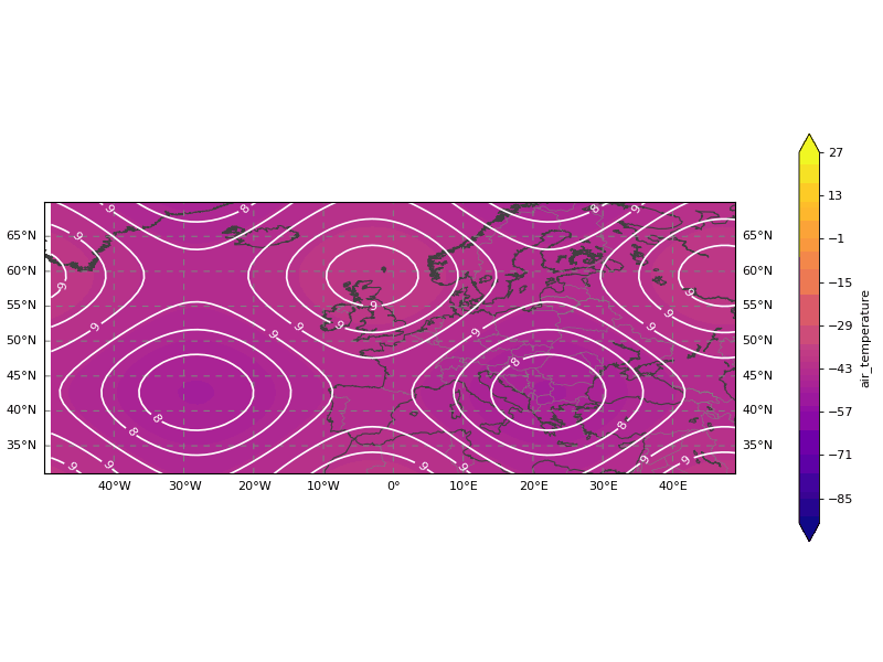
It produces the following plot, filled with a temperature colourmap and geopotential_height contour lines

By cutting the code into segments it will be easier to understand what it does and how to change it to your liking.

class HS_Template(mslib.mswms.mpl_hsec_styles.MPLBasemapHorizontalSectionStyle):
    name = "HSTemplate"  # Pick a proper camel case name starting with HS
    title = "Air Temperature with Geopotential Height"
    abstract = "Air Temperature (degC) with Geopotential Height (km) Contours"

We begin our plots with various identifiers and information which should be self-explanatory.

    required_datafields = [
        # level type, CF standard name, unit
        ("pl", "air_temperature", "degC"),
        ("pl", "geopotential_height", "km")
    ]

Within the required_datafields you list all quantities your plot initially needs as a list of 3-tuples containing

The type of vertical level (ml, pl, al, pv, tl, sfc)
The CF standard name of the entity required
The desired unit of the entity

    def _plot_style(self):
        fill_range = np.arange(-93, 28, 2)
        fill_entity = "air_temperature"
        contour_entity = "geopotential_height"

First inside the plotting function the desired range of the fill_entity is set. This will be the range of your colourmap. In this case the colourmap ranges between -93 and 28 °C in steps of 2. Adjust it to your liking. Second it is decided which entity will fill out the map and which will just be a contour above it. Of course you don’t need both, any one will suffice.

        # main plot
        cmap = mpl.cm.plasma

        cf = self.bm.contourf(
            self.lonmesh, self.latmesh, self.data[fill_entity],
            fill_range, cmap=cmap, extend="both")
        self.add_colorbar(cf, fill_entity)

Now the colourmap is decided, in this case “plasma”. It is best to pick one which best describes your data. Here is a list of all available ones. Afterwards the map is filled with the fill_entity and a corresponding colour bar is created. Of course if you only want a contour plot, you can delete this part of the code.

        # contour
        heights_c = self.bm.contour(
            self.lonmesh, self.latmesh, self.data[contour_entity], colors="white")
        self.bm.ax.clabel(heights_c, fmt="%i")

Lastly the contour_entity is drawn on top of the map, in white. Feel free to use any other colour. Of course if you don’t want a contour, you can delete this part of the code.

That’s about it. Feel free to download this template and play around with it however you like.

If you wish to include this into your WMS server

Put the file into your mswms_settings.py directory, e.g. ~/mss
Assuming you didn’t change the file or class name, append the following lines into your mswms_settings.py

from HS_template import HS_Template
register_horizontal_layers = [] if not register_horizontal_layers else register_horizontal_layers
register_horizontal_layers.append((HS_Template, [next(iter(data))]))